13 Mar 2015 by Fabian Hüske (@fhueske)
Join Processing in Apache Flink
Joins are prevalent operations in many data processing applications. Most data processing systems feature APIs that make joining data sets very easy. However, the internal algorithms for join processing are much more involved – especially if large data sets need to be efficiently handled. Therefore, join processing serves as a good example to discuss the salient design points and implementation details of a data processing system.
In this blog post, we cut through Apache Flink’s layered architecture and take a look at its internals with a focus on how it handles joins. Specifically, I will
- show how easy it is to join data sets using Flink’s fluent APIs,
- discuss basic distributed join strategies, Flink’s join implementations, and its memory management,
- talk about Flink’s optimizer that automatically chooses join strategies,
- show some performance numbers for joining data sets of different sizes, and finally
- briefly discuss joining of co-located and pre-sorted data sets.
Disclaimer: This blog post is exclusively about equi-joins. Whenever I say “join” in the following, I actually mean “equi-join”.
How do I join with Flink?
Flink provides fluent APIs in Java and Scala to write data flow programs. Flink’s APIs are centered around parallel data collections which are called data sets. data sets are processed by applying Transformations that compute new data sets. Flink’s transformations include Map and Reduce as known from MapReduce [1] but also operators for joining, co-grouping, and iterative processing. The documentation gives an overview of all available transformations [2].
Joining two Scala case class data sets is very easy as the following example shows:
// define your data types
case class PageVisit(url: String, ip: String, userId: Long)
case class User(id: Long, name: String, email: String, country: String)

// get your data from somewhere
val visits: DataSet[PageVisit] = ...
val users: DataSet[User] = ...

// filter the users data set
val germanUsers = users.filter((u) => u.country.equals("de"))
// join data sets
val germanVisits: DataSet[(PageVisit, User)] =
      // equi-join condition (PageVisit.userId = User.id)
     visits.join(germanUsers).where("userId").equalTo("id")
Flink’s APIs also allow to:
- apply a user-defined join function to each pair of joined elements instead returning a
($Left, $Right)tuple, - select fields of pairs of joined Tuple elements (projection), and
- define composite join keys such as
.where(“orderDate”, “zipCode”).equalTo(“date”, “zip”).
See the documentation for more details on Flink’s join features [3].
How does Flink join my data?
Flink uses techniques which are well known from parallel database systems to efficiently execute parallel joins. A join operator must establish all pairs of elements from its input data sets for which the join condition evaluates to true. In a standalone system, the most straight-forward implementation of a join is the so-called nested-loop join which builds the full Cartesian product and evaluates the join condition for each pair of elements. This strategy has quadratic complexity and does obviously not scale to large inputs.
In a distributed system joins are commonly processed in two steps:
- The data of both inputs is distributed across all parallel instances that participate in the join and
- each parallel instance performs a standard stand-alone join algorithm on its local partition of the overall data.
The distribution of data across parallel instances must ensure that each valid join pair can be locally built by exactly one instance. For both steps, there are multiple valid strategies that can be independently picked and which are favorable in different situations. In Flink terminology, the first phase is called Ship Strategy and the second phase Local Strategy. In the following I will describe Flink’s ship and local strategies to join two data sets R and S.
Ship Strategies
Flink features two ship strategies to establish a valid data partitioning for a join:
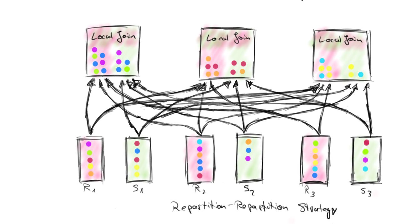
- the Repartition-Repartition strategy (RR) and
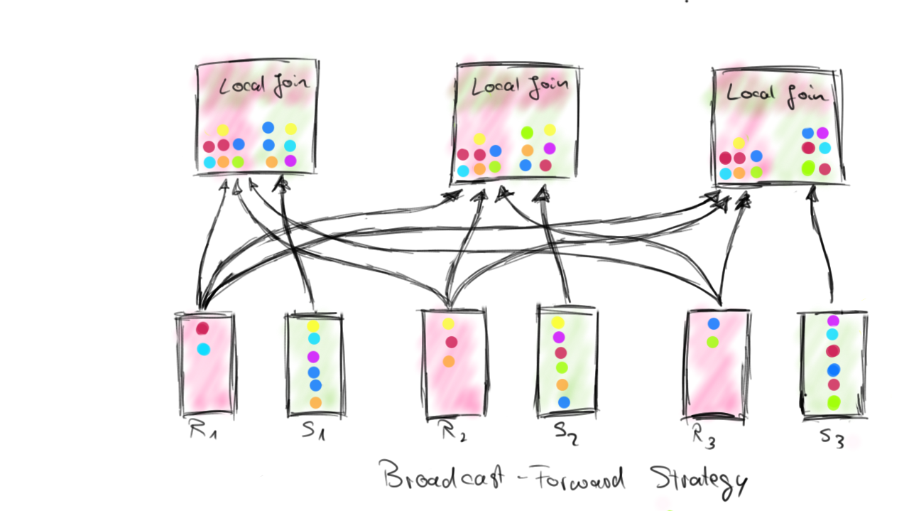
- the Broadcast-Forward strategy (BF).
The Repartition-Repartition strategy partitions both inputs, R and S, on their join key attributes using the same partitioning function. Each partition is assigned to exactly one parallel join instance and all data of that partition is sent to its associated instance. This ensures that all elements that share the same join key are shipped to the same parallel instance and can be locally joined. The cost of the RR strategy is a full shuffle of both data sets over the network.
The Broadcast-Forward strategy sends one complete data set (R) to each parallel instance that holds a partition of the other data set (S), i.e., each parallel instance receives the full data set R. Data set S remains local and is not shipped at all. The cost of the BF strategy depends on the size of R and the number of parallel instances it is shipped to. The size of S does not matter because S is not moved. The figure below illustrates how both ship strategies work.
The Repartition-Repartition and Broadcast-Forward ship strategies establish suitable data distributions to execute a distributed join. Depending on the operations that are applied before the join, one or even both inputs of a join are already distributed in a suitable way across parallel instances. In this case, Flink will reuse such distributions and only ship one or no input at all.
Flink’s Memory Management
Before delving into the details of Flink’s local join algorithms, I will briefly discuss Flink’s internal memory management. Data processing algorithms such as joining, grouping, and sorting need to hold portions of their input data in memory. While such algorithms perform best if there is enough memory available to hold all data, it is crucial to gracefully handle situations where the data size exceeds memory. Such situations are especially tricky in JVM-based systems such as Flink because the system needs to reliably recognize that it is short on memory. Failure to detect such situations can result in an OutOfMemoryException and kill the JVM.
Flink handles this challenge by actively managing its memory. When a worker node (TaskManager) is started, it allocates a fixed portion (70% by default) of the JVM’s heap memory that is available after initialization as 32KB byte arrays. These byte arrays are distributed as working memory to all algorithms that need to hold significant portions of data in memory. The algorithms receive their input data as Java data objects and serialize them into their working memory.
This design has several nice properties. First, the number of data objects on the JVM heap is much lower resulting in less garbage collection pressure. Second, objects on the heap have a certain space overhead and the binary representation is more compact. Especially data sets of many small elements benefit from that. Third, an algorithm knows exactly when the input data exceeds its working memory and can react by writing some of its filled byte arrays to the worker’s local filesystem. After the content of a byte array is written to disk, it can be reused to process more data. Reading data back into memory is as simple as reading the binary data from the local filesystem. The following figure illustrates Flink’s memory management.
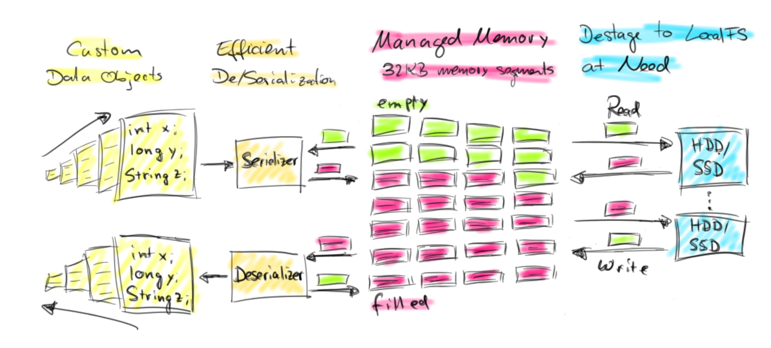
This active memory management makes Flink extremely robust for processing very large data sets on limited memory resources while preserving all benefits of in-memory processing if data is small enough to fit in-memory. De/serializing data into and from memory has a certain cost overhead compared to simply holding all data elements on the JVM’s heap. However, Flink features efficient custom de/serializers which also allow to perform certain operations such as comparisons directly on serialized data without deserializing data objects from memory.
Local Strategies
After the data has been distributed across all parallel join instances using either a Repartition-Repartition or Broadcast-Forward ship strategy, each instance runs a local join algorithm to join the elements of its local partition. Flink’s runtime features two common join strategies to perform these local joins:
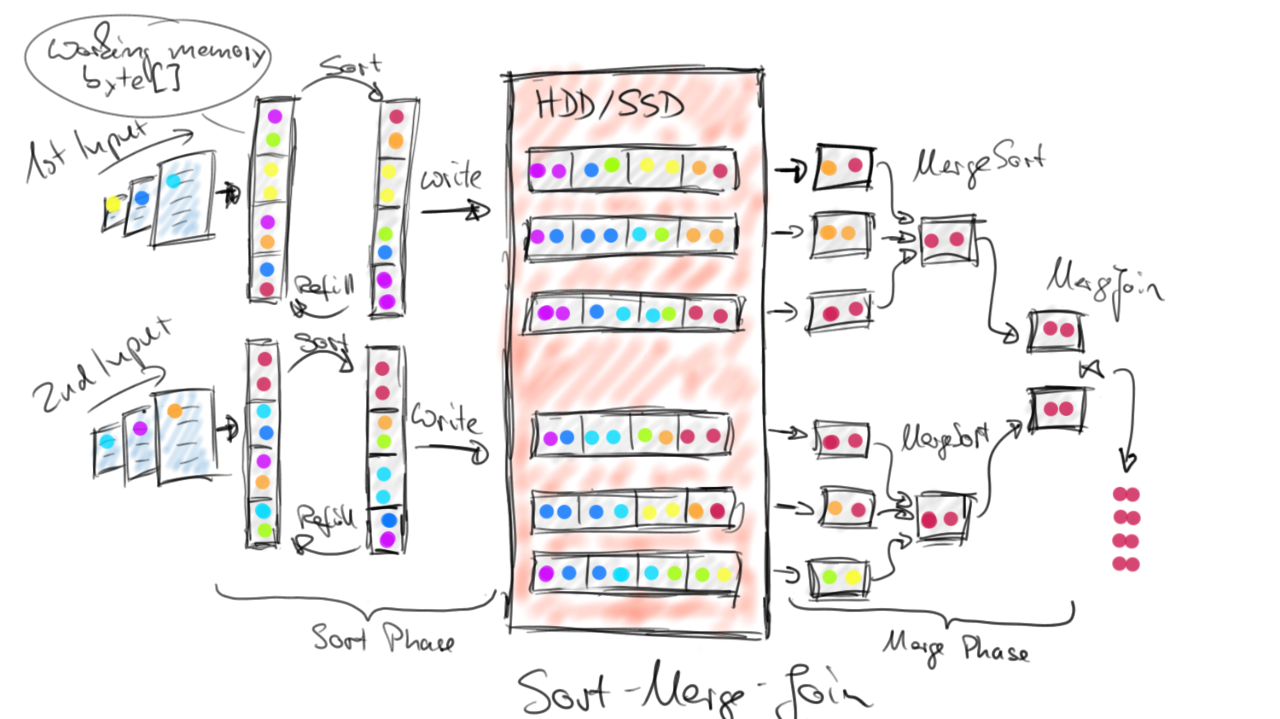
- the Sort-Merge-Join strategy (SM) and
- the Hybrid-Hash-Join strategy (HH).
The Sort-Merge-Join works by first sorting both input data sets on their join key attributes (Sort Phase) and merging the sorted data sets as a second step (Merge Phase). The sort is done in-memory if the local partition of a data set is small enough. Otherwise, an external merge-sort is done by collecting data until the working memory is filled, sorting it, writing the sorted data to the local filesystem, and starting over by filling the working memory again with more incoming data. After all input data has been received, sorted, and written as sorted runs to the local file system, a fully sorted stream can be obtained. This is done by reading the partially sorted runs from the local filesystem and sort-merging the records on the fly. Once the sorted streams of both inputs are available, both streams are sequentially read and merge-joined in a zig-zag fashion by comparing the sorted join key attributes, building join element pairs for matching keys, and advancing the sorted stream with the lower join key. The figure below shows how the Sort-Merge-Join strategy works.
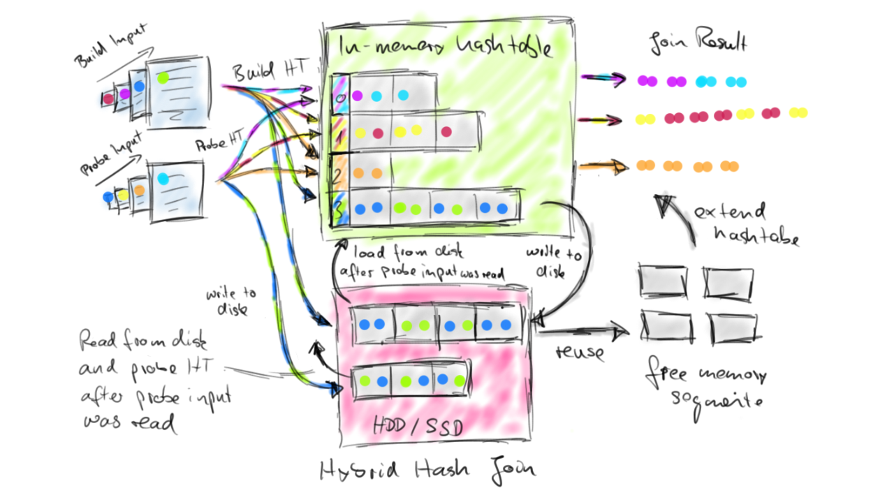
The Hybrid-Hash-Join distinguishes its inputs as build-side and probe-side input and works in two phases, a build phase followed by a probe phase. In the build phase, the algorithm reads the build-side input and inserts all data elements into an in-memory hash table indexed by their join key attributes. If the hash table outgrows the algorithm’s working memory, parts of the hash table (ranges of hash indexes) are written to the local filesystem. The build phase ends after the build-side input has been fully consumed. In the probe phase, the algorithm reads the probe-side input and probes the hash table for each element using its join key attribute. If the element falls into a hash index range that was spilled to disk, the element is also written to disk. Otherwise, the element is immediately joined with all matching elements from the hash table. If the hash table completely fits into the working memory, the join is finished after the probe-side input has been fully consumed. Otherwise, the current hash table is dropped and a new hash table is built using spilled parts of the build-side input. This hash table is probed by the corresponding parts of the spilled probe-side input. Eventually, all data is joined. Hybrid-Hash-Joins perform best if the hash table completely fits into the working memory because an arbitrarily large the probe-side input can be processed on-the-fly without materializing it. However even if build-side input does not fit into memory, the the Hybrid-Hash-Join has very nice properties. In this case, in-memory processing is partially preserved and only a fraction of the build-side and probe-side data needs to be written to and read from the local filesystem. The next figure illustrates how the Hybrid-Hash-Join works.
How does Flink choose join strategies?
Ship and local strategies do not depend on each other and can be independently chosen. Therefore, Flink can execute a join of two data sets R and S in nine different ways by combining any of the three ship strategies (RR, BF with R being broadcasted, BF with S being broadcasted) with any of the three local strategies (SM, HH with R being build-side, HH with S being build-side). Each of these strategy combinations results in different execution performance depending on the data sizes and the available amount of working memory. In case of a small data set R and a much larger data set S, broadcasting R and using it as build-side input of a Hybrid-Hash-Join is usually a good choice because the much larger data set S is not shipped and not materialized (given that the hash table completely fits into memory). If both data sets are rather large or the join is performed on many parallel instances, repartitioning both inputs is a robust choice.
Flink features a cost-based optimizer which automatically chooses the execution strategies for all operators including joins. Without going into the details of cost-based optimization, this is done by computing cost estimates for execution plans with different strategies and picking the plan with the least estimated costs. Thereby, the optimizer estimates the amount of data which is shipped over the the network and written to disk. If no reliable size estimates for the input data can be obtained, the optimizer falls back to robust default choices. A key feature of the optimizer is to reason about existing data properties. For example, if the data of one input is already partitioned in a suitable way, the generated candidate plans will not repartition this input. Hence, the choice of a RR ship strategy becomes more likely. The same applies for previously sorted data and the Sort-Merge-Join strategy. Flink programs can help the optimizer to reason about existing data properties by providing semantic information about user-defined functions [4]. While the optimizer is a killer feature of Flink, it can happen that a user knows better than the optimizer how to execute a specific join. Similar to relational database systems, Flink offers optimizer hints to tell the optimizer which join strategies to pick [5].
How is Flink’s join performance?
Alright, that sounds good, but how fast are joins in Flink? Let’s have a look. We start with a benchmark of the single-core performance of Flink’s Hybrid-Hash-Join implementation and run a Flink program that executes a Hybrid-Hash-Join with parallelism 1. We run the program on a n1-standard-2 Google Compute Engine instance (2 vCPUs, 7.5GB memory) with two locally attached SSDs. We give 4GB as working memory to the join. The join program generates 1KB records for both inputs on-the-fly, i.e., the data is not read from disk. We run 1:N (Primary-Key/Foreign-Key) joins and generate the smaller input with unique Integer join keys and the larger input with randomly chosen Integer join keys that fall into the key range of the smaller input. Hence, each tuple of the larger side joins with exactly one tuple of the smaller side. The result of the join is immediately discarded. We vary the size of the build-side input from 1 million to 12 million elements (1GB to 12GB). The probe-side input is kept constant at 64 million elements (64GB). The following chart shows the average execution time of three runs for each setup.
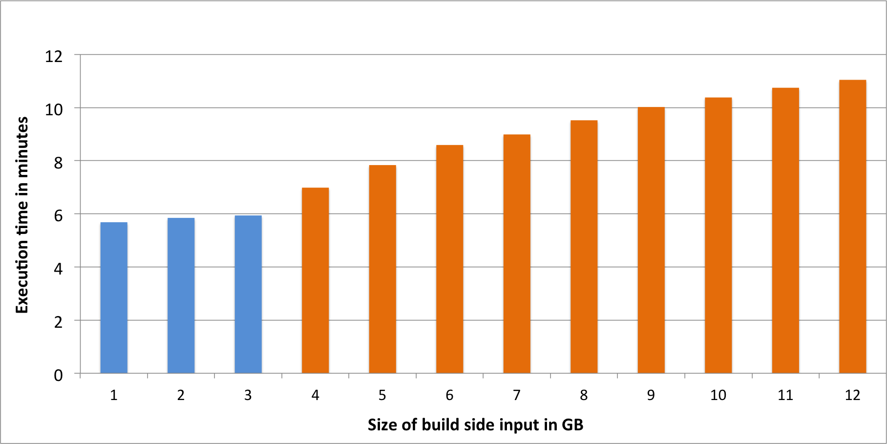
The joins with 1 to 3 GB build side (blue bars) are pure in-memory joins. The other joins partially spill data to disk (4 to 12GB, orange bars). The results show that the performance of Flink’s Hybrid-Hash-Join remains stable as long as the hash table completely fits into memory. As soon as the hash table becomes larger than the working memory, parts of the hash table and corresponding parts of the probe side are spilled to disk. The chart shows that the performance of the Hybrid-Hash-Join gracefully decreases in this situation, i.e., there is no sharp increase in runtime when the join starts spilling. In combination with Flink’s robust memory management, this execution behavior gives smooth performance without the need for fine-grained, data-dependent memory tuning.
So, Flink’s Hybrid-Hash-Join implementation performs well on a single thread even for limited memory resources, but how good is Flink’s performance when joining larger data sets in a distributed setting? For the next experiment we compare the performance of the most common join strategy combinations, namely:
- Broadcast-Forward, Hybrid-Hash-Join (broadcasting and building with the smaller side),
- Repartition, Hybrid-Hash-Join (building with the smaller side), and
- Repartition, Sort-Merge-Join
for different input size ratios:
- 1GB : 1000GB
- 10GB : 1000GB
- 100GB : 1000GB
- 1000GB : 1000GB
The Broadcast-Forward strategy is only executed for up to 10GB. Building a hash table from 100GB broadcasted data in 5GB working memory would result in spilling proximately 95GB (build input) + 950GB (probe input) in each parallel thread and require more than 8TB local disk storage on each machine.
As in the single-core benchmark, we run 1:N joins, generate the data on-the-fly, and immediately discard the result after the join. We run the benchmark on 10 n1-highmem-8 Google Compute Engine instances. Each instance is equipped with 8 cores, 52GB RAM, 40GB of which are configured as working memory (5GB per core), and one local SSD for spilling to disk. All benchmarks are performed using the same configuration, i.e., no fine tuning for the respective data sizes is done. The programs are executed with a parallelism of 80.
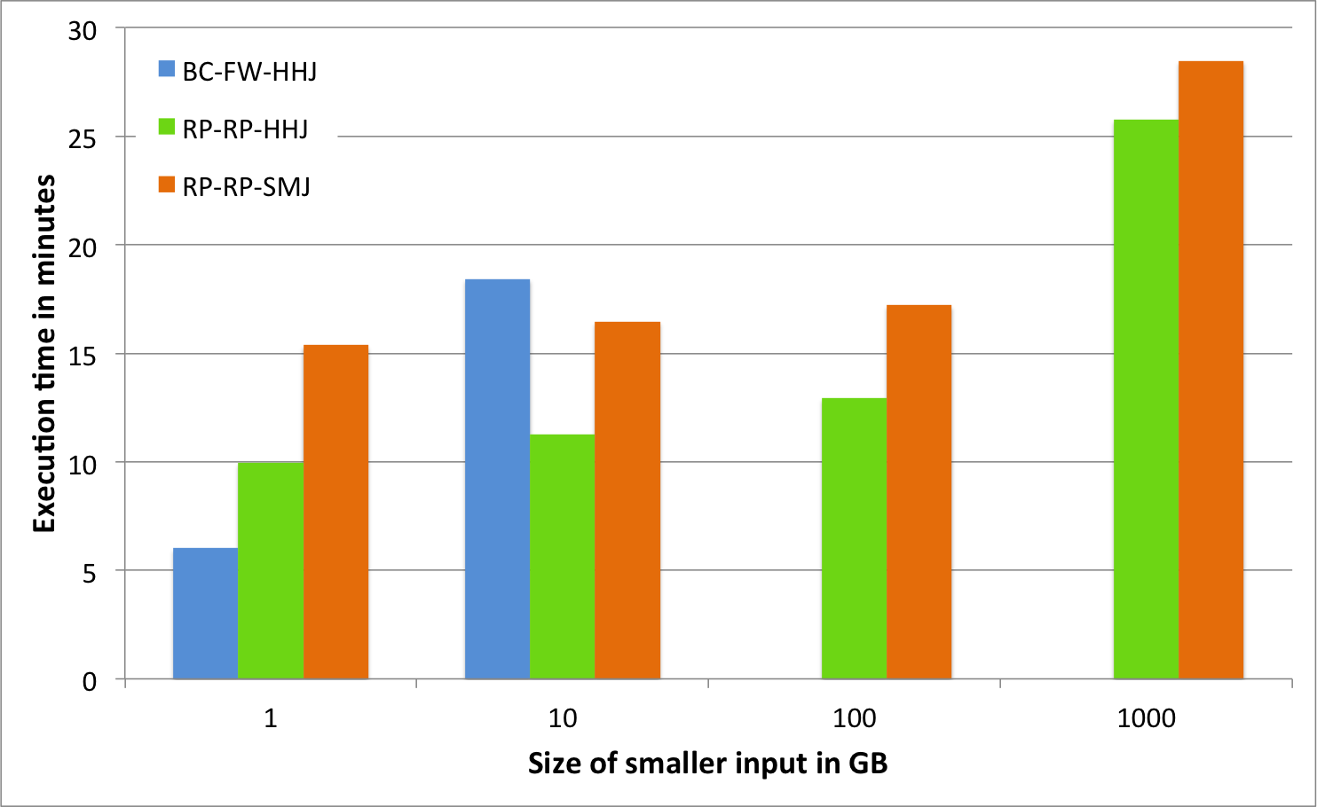
As expected, the Broadcast-Forward strategy performs best for very small inputs because the large probe side is not shipped over the network and is locally joined. However, when the size of the broadcasted side grows, two problems arise. First the amount of data which is shipped increases but also each parallel instance has to process the full broadcasted data set. The performance of both Repartitioning strategies behaves similar for growing input sizes which indicates that these strategies are mainly limited by the cost of the data transfer (at max 2TB are shipped over the network and joined). Although the Sort-Merge-Join strategy shows the worst performance all shown cases, it has a right to exist because it can nicely exploit sorted input data.
I’ve got sooo much data to join, do I really need to ship it?
We have seen that off-the-shelf distributed joins work really well in Flink. But what if your data is so huge that you do not want to shuffle it across your cluster? We recently added some features to Flink for specifying semantic properties (partitioning and sorting) on input splits and co-located reading of local input files. With these tools at hand, it is possible to join pre-partitioned data sets from your local filesystem without sending a single byte over your cluster’s network. If the input data is even pre-sorted, the join can be done as a Sort-Merge-Join without sorting, i.e., the join is essentially done on-the-fly. Exploiting co-location requires a very special setup though. Data needs to be stored on the local filesystem because HDFS does not feature data co-location and might move file blocks across data nodes. That means you need to take care of many things yourself which HDFS would have done for you, including replication to avoid data loss. On the other hand, performance gains of joining co-located and pre-sorted can be quite substantial.
tl;dr: What should I remember from all of this?
- Flink’s fluent Scala and Java APIs make joins and other data transformations easy as cake.
- The optimizer does the hard choices for you, but gives you control in case you know better.
- Flink’s join implementations perform very good in-memory and gracefully degrade when going to disk.
- Due to Flink’s robust memory management, there is no need for job- or data-specific memory tuning to avoid a nasty
OutOfMemoryException. It just runs out-of-the-box.
References
[1] “MapReduce: Simplified data processing on large clusters”, Dean, Ghemawat, 2004
[2] Flink 0.8.1 documentation: Data Transformations
[3] Flink 0.8.1 documentation: Joins
[4] Flink 1.0 documentation: Semantic annotations
[5] Flink 1.0 documentation: Optimizer join hints